Introduction
A probabilistic graphical model (PGM) consists of a probability distribution, defined on a set of variables, and a graph, such that each node in the graph represents a variable and the graph represents (some of) the independencies of the probability distribution. Some PGMs, such as Bayesian networks
[12], are purely probabilistic, while others, such as influence diagrams
[19], include decisions and utilities.
OpenMarkov (see
www.openmarkov.org) is an open source software tool developed at the Research Center on Intelligent Decision-Support Systems (
CISIAD) of the Universidad Nacional de Educación a Distancia (
UNED), in Madrid, Spain.
This tutorial explains how to edit and evaluate PGMs using OpenMarkov. It assumes that the reader is familiar with PGMs. An accessible treatment of PGMs can be found in the book by
[20]; other excellent books are
[4, 2, 22, 14, 16]. In Spanish, an introductory textbook to PGMs, freely available on internet, is
[8].
In this tutorial different fonts are used for different purposes:
-
Sans Serif is used for the elements of OpenMarkov’s graphical user interface (the menu bar, the network window, the OK button, the Options dialog...).
-
Emphasized style is used for generic arguments, such as the names of variables (Disease, Test...) and their values (present, absent...), types of networks (Bayesian network, influence diagram...), etc.
-
Bold is used for highlighting some concepts about probabilistic graphical models (finding, evidence...).
-
Typewriter is used for file names, extensions, and URLs (decide-therapy.pgmx, .csv, www.openmarkov.org...).
Finally, we should mention that the sections marked with an asterisk (for example, Sec.
3.3↓) are intended only for advanced users.
1 Bayesian networks: edition and inference
1.1 Overview of OpenMarkov’s GUI
This section offers a brief overview of OpenMarkov’s graphical user interface (GUI). The main screen has the following elements (see Figure
1.1↓):
-
The menu bar, which contains seven options: File, Edit, Inference, View, Window, Tools, and Help.
-
The first toolbar, located just under the menu bar, contains several icons for the main operations: Create new network (
 ), Open (
 ), Save (
 ), Load evidence (
 ), Zoom (
 ), Inference (
 ), and Decision tree (
 ). .
). .
-
The edit toolbar, located at the right of the first toolbar, contains six icons for several operations: Cut (
 ), Copy (
 ), Paste (
 ), Undo (
 ), and Redo (
 ), as well as five icons for choosing the edit tool, which may be one of the following:
-
Select object (
 );
);
-
Insert chance node (
 );
);
-
Insert decision node (
 );
);
-
Insert utility node (
 );
);
-
Insert link (
 ).
).
-
The network window is displayed below these toolbars. Figure 1.1↑ shows the network disease-test.pgmx, which will be used as a running example along this tutorial.
1.2 Editing a Bayesian network
We are going to solve the following problem using OpenMarkov.
For a disease whose prevalence is 8% there exists a test with a sensitivity of 75% and a specificity of 96%. What are the predictive values of the test for that disease?
In this problem there are two variables involved: Disease and Test. The disease has two values or states, present and absent, and the test can give two results: positive and negative. Since the first variable causally influences the second, we will draw a link Disease → Test.
1.2.1 Creation of the network
In order to create a network in OpenMarkov, click on the icon
Create a new network (

) in the first toolbar. This opens the
Network properties dialog. Observe that default network type is
Bayesian network and click
OK.
1.2.2 Structure of the network (graph)
In order to insert the nodes, click on the icon
Insert chance node (
) in the edit toolbar.
Then click on the point were you wish to place the node
Disease, as in Figure
1.1↑. Open the
Node properties window by double-clicking on this node. In the
Name field write
Disease. Click on the
Domain tab and check that the values that OpenMarkov has assigned by default are
present and
absent, which are just what we wished. Then click
OK to close the window.
Instead of creating a node and then opening the Node properties window, it is possible to do both operations at the same time by double-clicking on the point where we wish to create the node. Use this shortcut to create the node Test. After writing the Name of the node, Test, open the Domain tab, click Standard domains and select positive-negative. Then click OK.
Complete the graph by adding a link from the first node to the second: select the
Insert link tool (
) and drag the mouse from the origin node,
Disease, to the destiny,
Test. The result must be similar to Figure
1.1↑.
1.2.3 Saving the network
It is recommended to save the network on disk frequently, especially if you are a beginner in the use of OpenMarkov. The easiest way to do it is by clicking on the
Save network icon (

); given that this network has no name yet, OpenMarkov will prompt you for a
File name; type
disease-test and observe that OpenMarkov will add the extension
.pgmx to the file name, which stands for
Probabilistic Graphical Model in XML; it indicates that the network is encoded in
ProbModelXML, OpenMarkov’s default format (see
http://www.cisiad.uned.es/ProbModelXML). It is also possible to save a network by selecting the option
File ▷ Save as.
1.2.4 Selecting and moving nodes
If you wish to select a node, click on the
Selection tool icon (
) and then on the node. If you wish to select several nodes individually, press the
Control or
Shift key while clicking on them. It is also possible to select several nodes by dragging the mouse: the nodes whose center lies inside the rectangle drawn will be selected.
If you wish to move a node, click on the Selection tool icon and drag the node. It is also possible to move a set of selected nodes by dragging any of them.
1.2.5 Conditional probabilities
Once we have the nodes and links, we have to introduce the numerical probabilities. In the case of a Bayesian network, we must introduce a conditional probability table (CPT) for each node.
The CPT for the variable
Disease is given by its prevalence, which, according with the statement of the example, is
P(Disease=
present) = 0.08. We introduce this parameter by right-clicking on the
Disease node, selecting the
Edit probability item in the contextual menu, choosing
Table as the
Relation type, and introducing the value
0.08 in the corresponding cell. If we leave the edition of the cell (by clicking a different element in the same window or by pressing
Tab or
Enter), the value in the bottom cell changes to 0.92, because the sum of the probabilities must be one (see Figure
1.2↓).
The CPT for the variable
Test is built by taking into account that the sensitivity (75%) is the probability of a positive test result when the disease is present, and the specificity (96%) is the probability of a negative test result when the disease is absent (see Figure
1.3↓):
A shortcut for opening the potential associated to a node (either a probability or a utility potential) is to alt-click on the node.
1.3 Inference
Click the
Inference button (
) to switch from
edit mode to
inference mode. As the option
propagation is set to
automatic by default, OpenMarkov will compute and display the prior probability of the value of each variable, both graphically (by means of horizontal bars) and numerically---see Figure
1.4↓. Note that the
Edit toolbar has been replaced by the
Inference toolbar, whose buttons are described below.
1.3.1 Entering findings
A finding consists of the assignment of a value to a variable as a consequence of an observation. A set of findings is called an evidence case. The probabilities conditioned on a set of findings are called posterior probabilities.
For example, a finding may be the test has given a positive result:
Test =
positive. Introduce it by double-clicking on the state
positive of the node
Test (either on the string, or on the bar, or on the numerical value) and observe that the result is similar to Figure
1.5↓: the node
Test is colored in gray to denote the existence of a finding and the probabilities of its states have changed to 1.0 and 0.0 respectively. The probabilities of the node
Disease have changed as well, showing that
P(Disease=
present |
Test=
positive) = 0.6198 and
P(Disease=
absent |
Test=
positive) = 0.3802. Therefore we can answer the first question posed in Example
1.2↑: the
positive predictive value (PPV) of the test is \strikeout off\uuline off\uwave off61.98%.
An alternative way to introduce a finding would be to right-click on the node and select the Add finding option of the contextual menu. A finding can be removed by double-clicking on the corresponding value or by using the contextual menu. It is also possible to introduce a new finding that replaces the old one.
1.3.2 Comparing several evidence cases
In order to compute the
negative predictive value (NPV) of the test, create a new evidence case by clicking on the icon
Create a new evidence case (

) and introduce the finding {
Test =
negative}. The result must be similar to that of Figure
1.6↓. We observe that the NPV is
P(Disease=
absent |
Test=
negative) = 0.9779.
In this example we have two evidence cases: {
Test = positive} and {
Test = negative}. The probability bars and numeric values for the former are displayed in red and those for the second in blue.
1.4 Canonical models
Some probabilistic models are called
canonical because they can be used as elementary blocks for building more complex models
[12]. There are several types of canonical models:
OR,
AND,
MAX,
MIN, etc.
[7]. OpenMarkov is able to represent several canonical models and take profit of their properties to do the inference more efficiently. In order to see an example of a canonical model, follow these steps:
-
Build the network shown in Figure 1.7↓.
-
Open the potential for node E, set the Relation type to OR / MAX and introduce the values shown in Figure 1.8↓. The value 0.95 means that the probability that A causes E when the other parents of E are absent is 95%. The value 0.01 means that the probability that the causes of E not explicit in the model (i.e., the causes different from A, B, and C) produce E when the explicit causes are absent is 1%.
-
Select the radio button Whole table to make OpenMarkov show the conditional probability table for this node.
2 Learning Bayesian networks
2.1 Introduction
There are two main ways to build a Bayesian network. The first one is to do it
manually, with the help of a domain expert, defining a set of variables that will be represented by nodes in the graph and drawing causal arcs between them, as explained in Section
1.2↑. The second method to build a Bayesian network is to do it
automatically, learning the structure of the network (the directed graph) and its parameters (the conditional probabilities) from a dataset, as explained in Section
2.2↓.
There is a third approach,
interactive learning [10], in which an algorithm proposes some modifications of the network, called
edits (typically, the addition or the removal of a link), which can be accepted or rejected by the user based on their common sense, their expert knowledge or just their preferences; additionally, the user can modify the network at any moment using the graphical user interface and then resume the learning process with the edits suggested by the learning algorithm. It is also possible to use a
model network as the departure point of any learning algorithm, or just to indicate the positions of the nodes in the network learned, or to impose some links, etc. This approach is explained in Section
2.3↓.
When learning any type of model, it is always wise to gain insight about the dataset by inspecting it visually. The networks used in this chapter are in the format Comma Separated Values (CSV). They can be opened with a text editor, but this way it is very difficult to see the values of the variables. A better alternative is to use a spreadsheet, such as OpenOffice Calc or LibreOffice Calc. Microsoft Excel does not open these files properly because it assumes that in .csv files the values are separated by semicolons, not by commas; a workaround to this problem is to open the file with a text editor, replace the commas with semicolons, save it with a different name, and open it with Microsoft Excel.
2.2 Basic learning options
2.2.1 Automatic learning
In this first example we will learn the
Asia network
[17] with the hill climbing algorithm, also known as search-and-score
[6]. As a dataset we will use the file
asia10K.csv, which contains 10,000 cases randomly generated from the Bayesian network
http://www.cisiad.uned.es/ProbModelXML/networks (Figure
2.1↓).
-
Download onto your computer the file www.openmarkov.org/learning/datasets/asia10K.csv.
-
Open the dataset with a spreadsheet, as explained in Section 2.1↑.
-
In OpenMarkov, select the Tools ▷ Learning option. This will open the Learning dialog, as shown in Figure 2.2↓.
-
In the Database field, select the file asia10K.csv you have downloaded.
-
Observe that the default learning algorithm is Hill climbing and the default options for this algorithm are the metric K2 and a value of 0.5 for the α parameter, used to learn the numeric probabilities of the network (when α = 1, we have the Laplace correction). These values can be changed with the Options button.
-
Select Automatic learning and click Learn.
The learning algorithm builds the networks and OpenMarkov arranges the nodes in the graph in several layers so that all the links point downwards---see Figure
2.3↓.
2.2.2 Positioning the nodes with a model network
For those who are familiar with the
Asia network as presented in the literature
[17], it would be convenient to place the nodes of the network learned in the same positions as in Figure
2.1↑ to see more easily which links differ from those in the original network. One possibility is to drag the nodes after the network has been learned. Another possibility is to make OpenMarkov place the nodes as in the original network; the process is as follows:
-
Download the network http://www.probmodelxml.org/networks/bn/BN-asia.pgmx.
-
Open the dataset asia10K.csv, as in the previous example.
-
Select Automatic learning.
-
In the Model network tab, select Load model network from file, click Open and select your file BN-asia.pgmx.
-
Select Use the information of the nodes.
-
Click Learn.
The network learned, shown in Figure
2.4↓, has the same links as in Figure
2.3↑ but the nodes are in the same positions as in Figure
2.1↑.
The facility for positioning the nodes as in the model network is very useful even when we do
not have a network from which the data has been generated: if we wish to learn several networks from the same dataset---for example by using different learning algorithms or different parameters---we drag the nodes of the first network learned to the positions that are more intuitive for us and then use it as a model for learning the other networks; this way all of them will have their nodes in the same positions.
2.2.3 Discretization and selection of variables
In OpenMarkov there are three options for preprocessing the dataset:
-
selecting the variables to be used for learning,
-
discretizing the numeric variables (or some of them), and
-
treating missing values.
In this example we will illustrate the first two options; the third one is explained in Section
2.2.4↓.
-
Download the dataset Wisconsin Breast Cancer (file www.openmarkov.org/learning/datasets/wdbc.csv), which has been borrowed from the UCI Machine Learning Repository (see http://archive.ics.uci.edu/ml/datasets/Breast+Cancer+Wisconsin+%28Diagnostic%29).
-
Open it with a spreadsheet and observe that all the variables are numeric except Diagnosis.
-
Open it in OpenMarkov’s Learning dialog.
-
Select Automatic learning.
-
In the tab Preprocessing, select Use selected variables and and uncheck the box of the variable ID, as shown in Figure 2.5↓. (Many medical databases contain administrative variables, such as the patient ID, the date of admission to hospital, the room number, etc., which are irrelevant for diagnosis and therefore should be excluded when learning a model.) If we had specified a model network, the option Use only the variables in the model network would be enabled.
-
In the Discretize field, common to all variables, select Equal width intervals, check the box Same number of intervals and increase the Number of intervals to 3. This means that every numeric variable will be discretized into three intervals of equal width, as we will verify after learning the network.
-
Observe that the discretization combo box for the variable Diagnosis in the column Discretization says Do not discretize---even though in the Discretize field, common to all the variables, we have chosen Equal width intervals---because this variable is not numeric and hence cannot be discretized.
-
Click Learn. The result is shown in Figure 2.6↓.
-
At the Domain tab of the Node properties dialog of the node RadiusMean (placed at the lower left corner in the graph), observe that this variable has three states, as shown in Figure 2.7↓, corresponding to three intervals of the same width; the minimum of the first interval, 6.981, is the maximum value for this variable in the dataset, and the maximum of the third interval, 28.11) is the maximum in the dataset---as you can easily check.
-
Repeat the previous step several times to examine the domains of the other numeric variables of the network learned.
2.2.4 Treatment of missing values
This example explains the two rudimentary options that OpenMarkov offers currently for dealing with missing values: the option Erase records with missing values ignores every register that contains at least one missing value, while the option Keep records with missing values fills every empty cell in the dataset with the string “missing”, which is then treated as if it were an ordinary value. The drawback of the first one is that it may leave too few records in the dataset, thus making the learning process completely unreliable. A drawback of the second option is that assigning the string “missing” to a numeric variable converts it into a finite-state variable, which implies that each numeric value will be treated as a different state; it is also problematic when using a model network, because in general this network does not have the state “missing” and in any case this state would have a different meaning.
In the following example we will use a combination of both options: for the two variables having many missing values (workclass and occupation) we will select the option Keep records with missing values, because the other option would remove too many records; for the other variables we will select the option Erase records with missing values, which will remove only 583 cases, namely 2% of the the records in the dataset.
-
Download the Adult dataset (www.openmarkov.org/learning/datasets/adult.csv), which has also been borrowed from the UCI Machine Learning Repository (see http://archive.ics.uci.edu/ml/datasets/Adult).
-
Open it with a spreadsheet and observe that most missing values are located on the variables workclass and occupation.
-
Open it with OpenMarkov’s Learning dialog.
-
Select Automatic learning.
-
Switch to the Preprocessing tab. In the Discretize field select Equal width intervals; check the box for Same number of intervals and increase the Number of intervals to 3. In the list of variables, observe that the content of the Discretization column is Equal width intervals for the 6 numeric variables and Do not discretize for the 9 finite-state variables.
-
Observe that the default value of the field Treat missing values is Specify for each variable.
-
In the Missing values column, select Erase records with missing values for all variables except workclass and occupation, as mentioned above.
-
Click Learn. The result is shown in Figure 2.8↓.
2.3 Interactive learning
In the previous section we have explained the main options for learning Bayesian networks with OpenMarkov, which are common for automatic and interactive learning. In this section we describe the specific options for interactive learning.
2.3.1 Learning with the hill climbing algorithm
In this first example we will learn the
Asia network with the
hill climbing algorithm, as we did in Section
2.2.1↑, but in this case we will do it interactively.
-
Open the dataset asia10K.csv.
-
Observe that by default the Learning type is Interactive learning.
-
Click Learn. You will see a screen similar to the one in Figure 2.9↓. Observe that OpenMarkov has arranged the nodes in a circle to facilitate the visualization of the links during the leaning process. The Interactive learning window shows the score of each edit---let us remember that we are using the metric K2. Given that the hill climbing algorithm departs from an empty network, the only possible edits are the addition of links.
-
If we clicked Apply edit, OpenMarkov would execute the first edit in the list, namely the addition of the link Dyspnea → Bronchitis. However, bronchitis is a disease and dyspnea is a symptom. Therefore, it seems more intuitive to choose instead the second edit proposed by the learning algorithm, namely the addition of the link Bronchitis → Dyspnea, whose score is almost as high of that of the first. Do it by either selecting the second edit and clicking Apply edit or by double-clicking on it.
-
Observe that after adding the link Bronchitis → Dyspnea, OpenMarkov generates the list of possible edits for the new network and recomputes the scores.
-
Click Apply edit to select the first edit in the list, which is the addition of the link LungCancer → TuberculosisOrCancer. The reason for this link is that when LungCancer is true then TuberculosisOrCancer is necessarily true.
-
For the same reason, the network must contain a link Tuberculosis → TuberculosisOrCancer. Draw it by selecting the Insert link tool (
) and dragging from Tuberculosis to TuberculosisOrCancer on the graph. Observe that OpenMarkov has updated again the list of edits even though this change has been made on the graph instead of on the list of edits.
-
Click Complete phase or Finish to terminate the algorithm, i.e., to iterate the search-and-score process until there remains no edit having a positive score. In this case, in which the algorithm has only one phase, the only difference between these two buttons is that Finish closes the Interactive learning window.
2.3.2 Imposing links with a model network
There is another use of the model network that can be applied also in automatic learning, but we explain it here because its operation is more clear in interactive learning. We will also use the following example to illustrate two additional options of interactive learning: Only allowed edits and Only positive edits.
Assuming that you wish to impose that the network learned has the links LungCancer → TuberculosisOrCancer and Tuberculosis → TuberculosisOrCancer, whatever the content of the dataset, proceed as follows:
-
Open the Bayesian network BN-asia.pgmx.
-
Remove all the other links, as in Figure 2.10↓.
-
Open the dataset asia10K.csv.
-
In the Model network tab, select Use the network already opened and Start learning from model network.
-
Uncheck the boxes Allow link removal and Allow link inversion. Leave the box Allow link addition checked.
-
Click Learn.
-
In the Interactive learning window, uncheck the box Only allowed edits. Observe that a new edit is added on top of the list: the addition of link TuberculosisOrCancer → Tuberculosis, which is not allowed because it would create a cycle in the Bayesian network. Check this box again.
-
In the same window, uncheck the box Only positive edits. Click Apply edit six times. Observe that some edits having negative scores are shown at the end of the list. Check that box again.
-
Click Finish.
2.3.3 Learning with the PC algorithm
Finally, we will learn a network from the
asia10K.csv dataset using the
PC algorithm
[18] to observe how it differs from
hill climbing. In order to understand the following example, let us remember that the PC algorithm departs from a fully-connected undirected network and removes every link that is not supported by the data. If two variables,
X and
Y, are independent, i.e., if the correlation between them is 0, then the link
X--
Y is removed. If there is some correlation, a statistical test of independence is performed to decide whether this correlation is authentic (i.e., a property of the general population from which the data was drawn) or spurious (i.e., due to the hazard, which is more likely in the case of small datasets). The null hypothesis (
H0) is that the variables are conditionally independent and, consequently, the link
X--
Y can be removed. The test returns a value,
p, which is the likelihood of
H0. When
p is smaller than a certain value, called
significance level and denoted by
α, we reject
H0, i.e., we conclude that the correlation is authentic and keep the link
X--
Y. In contrast, when
p is above the threshold
α we cannot discard the null hypothesis, i.e., we maintain our assumption that the variables are independent and, consequently, remove the link
X--
Y. The higher the
p, the more confident we are when removing the link. The PC algorithm performs several tests of independence; first, it examines every pair of variables
{X, Y} with no conditioning variables, then with one conditioning variable, and so on.
The second phase of the algorithm consists of orienting some pairs of links head-to-head in accordance with the results of the test of independence, as explained below. Finally, in the third phase the rest of the links are oriented one by one.
In this example we apply the PC algorithm to the dataset asia10K, which we have already used several times in this chapter.
-
Open the dataset asia10K.csv.
-
Select the PC algorithm. Observe that by default the independence test is Cross entropy and the significance level is 0.05.
-
Click Learn. Observe that this algorithm departs from a completely connected undirected network, as shown in Figure 2.11↓. In the first phase of the algorithm, each edit shown in the Interactive learning window consists of removing a link due to a relation of conditional independence; the motivation of each edit shows the conditioning variables (within curly brackets) and the p-value returned by the test. The list of edits shows first the relations in which there is no conditioning variable; in this case, there are 7 relations. Within this group, the edits having higher p-values are shown at the top of the list, because these are the links we can remove more confidently.
-
Observe that for all these edits the p-value is above the threshold 0.05. If the checkbox Only positive edit were unchecked, the list would also include the edits having a p-value smaller than the threshold; in this example, there are 6 edits with p = 0.000. Of course, it does not make sense to apply those edits. Therefore, we should keep the box checked.
-
Click Apply edit 7 times to execute the edits corresponding to no conditioning variables.
-
Observe that now the first edit proposed is to remove the link VisitToAsia − TuberculosisOrCancer; its motivation is “{Tuberculosis} p: 0.9981”, which means that VisitToAsia and TuberculosisOrCancer are conditionally independent given Tuberculosis---more precisely, that the test aimed at detecting the correlation between them, conditioned on Tuberculosis, has returned a p-value of 0.9981, which is also above the significance level.
-
Click Apply edit 12 times to execute the edits corresponding to one conditioning variable. Now you may click Apply edit 3 times to execute the edits corresponding to two conditioning variables. Alternatively, you may click Complete phase to execute all the remove-link edits. (If you click Apply edit when there is only one remaining edit in the current phase, OpenMarkov automatically proceeds to the next phase after executing it.)
-
The second phase of the algorithm consists of orienting some pairs of links head-to-head based on the tests of independence carried out in the first phase [12, 18]. You can execute those edits one by one or click Complete phase to proceed to third phase, in which the rest of the links will be oriented. It also possible to click Finish at any moment to make the algorithm run automatically until it completes its execution.
2.4 Exercises
As an exercise, we invite you to experiment with the Asia dataset using different significance levels for the PC algorithm, different metrics for the hill climbing algorithm, different model networks to impose or forbid some links, etc., and compare the resulting networks. You can also try blocking and unblocking some of the edits proposed by the algorithm (with the buttons Block edit and Show blocked), selecting other edits than those on the top of the list, adding or removing some links on the graph, etc.
You can also experiment with the
Alarm dataset (
www.openmarkov.org/learning/datasets/alarm10K.csv), which contains 10,000 records randomly generated from the
Alarm network
[9], a very famous example often used in the literature on learning Bayesian networks.
Finally, you can use your favorite network, generate a dataset by sampling from it (Tools ▷ Generate database) and try to learn it back with different algorithms.
3 Influence diagrams
3.1 A basic example
In order to explain the edition and evaluation of influence diagrams in OpenMarkov, let us consider the following example.
The effectiveness (measured in a certain scale) of the therapy for the disease mentioned in Example
1.2↑ is shown in Table
3.1↓. The test is always performed before deciding about the therapy. In what cases should the therapy be applied?
|
|
Disease=absent
|
Disease=present
|
|
Therapy=yes
|
9
|
8
|
|
Therapy=no
|
10
|
3
|
Table 3.1 Effectiveness of the therapy.
In Table
3.1↑ we observe that the best scenario is that the disease is absent and no therapy is applied (effectiveness = 10). The worst scenario is that a patient suffering from the disease does not receive the therapy (effectiveness = 3). If a sick person receives the therapy the effectiveness increases to 8. If a healthy person receives the therapy the effectiveness decreases to 9 as a consequence of the side effects. The problem is that we do not know with certainty whether the disease is present or not, we only know the result of the test, which sometimes gives false positives and false negatives. For this reason we will build an influence diagram to find out the best intervention in each case.
3.1.1 Editing the influence diagram
The edition of influence diagrams is similar to that of Bayesian networks. The main difference is that now the icons for inserting decision nodes and utility nodes are enabled, as shown in Figure
3.1↓. It would be possible to build an influence diagram for our problem from scratch. However, it is better to depart from the Bayesian network built for the Example
1.2↑ in Section
1.2↑ and convert it into an influence diagram.
-
Open the network disease-test.pgmx. Open its contextual menu by right-clicking on the background of the network, click Network properties, and in the Network type field select Influence diagram. Observe that the icons for inserting decision nodes (
) and utility nodes (
) are now active.
-
Click on the Insert decision node icon and double-click on the place where you wish to insert the Therapy node. In the Name field type Therapy. Click on the Domain tab and check that the values (states) are yes and no; these are OpenMarkov’s default values for decision nodes.
-
Click on the Insert utility node icon, double-click on the place where you wish to insert the Effectiveness node, and in the Name field type Effectiveness.
-
Draw the links Disease → Effectiveness and Test → Effectiveness because, according with Table 3.1↑, the effectiveness depends on Disease and Therapy. Draw the link Test → Therapy because the result of the test is known when making the decision about applying the therapy or not; the links that indicate which findings are available when making a decision are called informational arcs. The result should be similar to that in Figure 3.1↑.
-
Open the potential for the node Effectiveness by selecting Edit utility in the contextual menu or by alt-clicking on the node. In the Relation type field select Table. Introduce the values given in Table 3.1↑, as shown in Figure 3.2↓.
In this moment the nodes Disease and Test have the potentials we assigned to them when building the Bayesian network, namely, a conditional probability table for each node. The utility node has the potential we have just assigned to it. The node Therapy does not need any potential because it is a decision. Therefore, the influence diagram is complete. Save it in the file decide-therapy.pgmx.
3.1.2 Optimal strategy and maximum expected utility
The values that are known making a decision are known as its
informational predecessors. In this case, the only informational predecessor of the decision
Therapy is
Test. A
policy for a decision is a family of probability distributions for the options of the decision, such that there is one distribution for each configuration of its informational predecessors. For example, the policy shown in Figure
3.3↓ contains two probability distributions, one for
Test =
negative and another one for
Test =
positive. The former states that when the test gives a negative result, the option
no (do not apply the therapy) will be always chosen (probability = 1.0 = 100%). Similarly, the probability distribution for
Test =
positive means that when the test gives a positive result the option
yes (apply therapy) will always be chosen. The reason why some cells in Figure
3.3↓ are colored in red in will be explained below. A policy in which every probability is either 0 or 1, as in this example, is called a
deterministic policy. It is also possible to have purely probabilistic policies, i.e., those in which some of the probabilities are different from 0 and 1.
A strategy is a set of policies, one for each decision in the influence diagram. Each strategy has a expected utility, which depends on the probabilities and utilities that define the influence diagram and on the policies that constitute the strategy. A strategy that maximizes the expected utility is said to be optimal. A policy is said to be optimal if it makes part of an optimal strategy.
The resolution of an influence diagram consists of finding an optimal strategy and its expected utility, which is the maximum expected utility.
In order to evaluate the influence diagram built above, click the
Inference button (
) to switch from
edit mode to
inference mode. OpenMarkov performs two operations: the first one, called
resolution, consists of finding the optimal strategy, as we have just explained. The policies that constitute the optimal strategy can be inspected at the corresponding decision nodes. In the contextual menu of the node
Therapy, select
Show optimal policy. It will open the window shown in Figure
3.3↑. For each column (i.e., for each configuration of the informational predecessors of this node), the cell corresponding to the optimal option is colored in red.
The second operation performed by OpenMarkov when switching to inference mode, called
propagation, consists of computing the posterior probability of each chance and decision node and the expected utility of each utility node. The result is shown in Figure
3.4↓. As this influence diagram contains only one utility node, the value
9.
7032 shown therein is the global maximum expected utility of the influence diagram.
3.2 An example involving two decisions
In this section we introduce an example involving two decisions. It will help us explain the concept of
super-value node [11] and, later, how to introduce evidence in influence diagrams (Sec.
3.3↓) and how to impose policies (Sec.
3.4↓).
The test mentioned in the Example
1.2↑ has a cost of 0.2 (measured in the same scale as the effectiveness shown in Table
3.1↑---Example
3.1↑). Is it worth doing the test? Put another way, the test will give us useful information for deciding when to apply the therapy, but the question is whether this benefit outweighs the cost of the test.
3.2.1 Construction of the influence diagram
This problem can be solved by building the influence diagram shown in Figure
3.5↓. The steps necessary to adapt the previous influence diagram,
decide-therapy.pgmx, are the following:
-
Create the node Dec:Test, which represents the decision of doing the test or not.
-
Create the nodes Cost of test and Global utility. The latter is called a super-value node because its parents are other utility nodes.
-
Draw the links Dec:Test → Test, Dec:Test → Cost of test, Effectiveness → Global utility, and Cost of test → Global utility.
-
At the Domain tab of the Node properties dialog for the node Test, add the state not done (Figure 3.6↓).
-
Introduce the numerical values of the conditional probability table for the node Test, as shown in Figure 3.7↓. It may be necessary to use the Reorder variables option.
-
Introduce the numerical values of the utility table for Cost of test, as in Figure 3.8↓. Note that the cost is introduced as a negative utility.
-
Check that the utility potential for the node Global utility is of type Sum, which means that the global utility is the sum of the effectiveness and (the opposite of) the cost of the test.
-
Save this influence diagram as decide-test.pgmx.
In this example the node Global utility is not strictly necessary, because when an influence diagram contains several utility nodes that do not have children, OpenMarkov assumes that the global utility is the sum of them; in this case, the global utility would be the sum of Effectiveness and Cost of test even if we had not added the node Global utility. The optimal policies, the posterior probabilities, and the expected utilities would be exactly the same.
3.2.2 Evaluation of the influence diagram
Let us now evaluate the influence diagram and examine all the information that OpenMarkov offers us.
-
Click on the Inference icon. The result is shown in Figure 3.9↓.
-
We examine first the policies that constitute the optimal strategy. Observe that the optimal policy for Dec:Test is to always do the test (Figure 3.10↓).
-
Examine the optimal policy for Therapy, shown in Figure 3.11↓. In that table, the last column means that the therapy should be applied when the test is done and gives a positive result. The penultimate column indicates that the therapy should not be applied when the test is done and gives a negative result.
There are three columns that indicate “apply the therapy in 50% of cases, do not in the other 50%”. The reason for this is that, as there was a tie in the expected utilities, OpenMarkov has made the Solomonic decision of not favoring any of the two options: half the patients should receive the therapy, half should not. However, the content of these columns is irrelevant because they correspond to impossible scenarios: two of them, {
Dec:Test =
no,
Test =
negative} and {
Dec:Test =
no,
Test =
positive}, are impossible, because when the test is not done it gives neither a positive nor a negative result---see Figure
3.7↑; the scenario {
Dec:Test =
yes,
Test =
not done} is also impossible due to an obvious contradiction---see again Figure
3.7↑.
The first column means that if the test were not done, the best option would be not to apply the therapy. However, this scenario is also impossible because the optimal strategy implies doing the test in all cases.
-
After having examined the policies, we analyze the posterior probabilities and the expected utilities shown in Figure 3.9↑. Observe at the node Dec:Test that the test will be done in 100% of cases; this is a consequence of the optimal policy for this decision (Figure 3.10↑).
-
Observe at the node Therapy that 9.68% of patients will receive the therapy, exactly the same proportion that will give a positive result in the test (see the node Test). This coincidence is a result of the policy for the node Therapy, namely to apply the therapy if and only if the test gives a positive result (see Figure 3.11↑).
-
The expected utility of Cost of test is − 0.2, a consequence of the policy of doing the test in all cases.
-
The expected utility of Effectiveness is 9.7032, the same as in Example 3.1↑ (Figure 3.4↑) in which the test was always done.
-
The Global utility is 9.5032, just the sum of the other utilities: 9.7032 + ( − 0.2).
3.3 Introducing evidence in influence diagrams*
This section, intended only for advanced users, describes the difference between the two kinds of findings for influence diagrams in OpenMarkov: pre-resolution and post-resolution.
3.3.1 Post-resolution findings
In the scenario of Example
3.2↑, what is the expected utility for the patients suffering from the disease?
This question can be answered with the influence diagram
decide-test.pgmx by
first evaluating it and
then introducing the finding
Disease =
present, as we did with Bayesian networks (Sec.
1.3.1↑). The result, shown in Figure
3.12↓, is that the test will give a positive result in 75% of cases (in accordance with the sensitivity of the test) and a negative result in the rest. We can also see that 75% of those patients will receive the therapy, as expected from the policy for
Therapy. We can also see that the expected value of
Effectiveness is 6.75; it is the result of a weighted average, because the effectiveness is 8 for those having a positive test and 3 for those having a negative test (see Table
3.1↑):
8 × 0.75 + 3 × 0.25 = 6.75. Finally, the answer to the above question is that the expected utility for those patients is 6.55.
In the scenario of Example
3.2↑, what is the probability that of suffering from the disease when the test gives a positive result?
This question can also be answered with the influence diagram
decide-test.pgmx in a similar way, i.e., introducing the post-resolution finding
Test =
positive, as in Figure
3.13↓, where we can see that the probability of suffering from the disease when the test gives a positive result (a true positive) is 61.98%. This answers the question under consideration. We can further analyze that figure and observe that 100% of the patients with a positive test will receive the therapy and that their expected effectiveness is 8.3802, which is the weighted average of true positives and false positives:
8 × 0.6198 + 9 × 0.3802 = 8.3802. The expected utility is the effectiveness minus the cost of the test, 8.1832.
3.3.2 Pre-resolution findings
Given the problem described in Example
3.2↑, what would be the optimal strategy if the decision maker---the doctor, in this case---knew with certainty that some patient has the disease?
One way to solve this problem with OpenMarkov is to use the influence diagram
decide-test.pgmx built above, but introducing the finding
Disease =
present before evaluating this influence diagram---for this reason it is called a
pre-resolution finding. This can be accomplished by using the
Add finding option of the contextual menu of the node
Disease in edit mode and
then evaluating the influence diagram---see Figure
3.14↓. The optimal strategy computed by OpenMarkov is “apply the therapy without testing”. This explains why the probability of
Dec:Test =
yes is 0 in this diagram, while it was 1 in Figure
3.12↑.
Another difference is that the node
Disease in Figure
3.14↑ is colored in dark gray to indicate that it has a pre-resolution finding, while the lighter gray in Figure
3.12↑ denotes a post-resolution finding.
The main difference between the Examples
3.3.1↑ and
3.3.2↑ is that in the latter the decision maker (the doctor) knows that the patient has the disease before making the decisions about the test and the therapy---this is what a pre-resolution finding means---and for this reason he/she does not need to do the test, while if in the Example
3.3.2↑ the doctor has decided to do the test to all patients because he/she did not know with certainty who has the disease. The question posed in that example takes the perspective of an external observer who, knowing the decision maker’s strategy, i.e., how he/she will behave, uses the influence diagram---the model---to compute the posterior probabilities and the expected utilities for different subpopulations. Therefore the strategy does not depend on the information known by the external observer, which is unknown to the decision maker.
Pre-resolution findings, which are known to the decision maker since the beginning, i.e., before making any decision, correspond to concept of evidence defined in
[15], while post-resolution findings correspond to the concept of evidence proposed in
[3].
3.4 Imposing policies*
OpenMarkov allows the user to impose policies on decision nodes. The decisions that have imposed policies are treated as if they were chance nodes, i.e., when the evaluation algorithm looks for the optimal strategy it only returns optimal policies for those decisions that do not have imposed policies, and these returned policies, which are optimal in the context of the policies imposed by the user, may differ from the absolutely optimal policies.
The purpose of imposing policies is to analyze the behavior of the influence diagram for scenarios that can never occur if the decision maker applies the optimal strategy.
Let us consider again the problem defined in the Example
3.2↑, in which there is a disease, a test, and a therapy, but now assuming that the cost of the test is 0.4 instead of 0.2. In this case, the optimal strategy would be “no test, no therapy”. However, we may wonder---as we did en Example
3.3.1↑---what would be the posterior probability of
Disease depending on the result of the test.
In order to solve this problem, build a new influence diagram, decide-test-high-cost.pgmx, which will be identical to decide-test.pgmx except in the cost of the test:
-
If you still have the influence diagram decide-test.pgmx in the state shown in Figure 3.14↑, return to edit mode by clicking on the Inference icon and, in the contextual menu of the node Disease, select the option Remove finding. Otherwise, open again the file decide-test.pgmx.
-
Edit the utility table of Cost of test and write − 0.4 instead of − 0.2 in the column yes.
-
Save the influence diagram as decide-test-high-cost.pgmx.
-
Click on the Inference icon. Observe that now the optimal policy for Dec:Test is to never do the test.
-
Double-click on the state positive of the node Test to observe the posterior probabilities of Disease.
The result is that OpenMarkov gives an error message, “Incompatible evidence”, because the test cannot give a positive result when it is not done. Then we can say: “OK, I know the optimal policy is not to do the test, but what would happen if, applying a non-optimal policy, I decided to do it?”, which is the question posed in the statement of this example. This kind of what-if reasoning can be performed by following these steps:
-
Come back to edit mode by clicking on the Inference icon, because policies can only be imposed in edit mode.
-
In the contextual menu of Dec:Test, select Impose policy. In the field Relation type, select Table and introduce the values shown in Figure 3.15↓. This imposed policy means that 100% of patients will receive the test.
-
Click OK and observe that the node Dec:Test is now colored in a darker blue, to indicate that it has an imposed policy.
-
Evaluate the influence diagram. Observe that now the probability of doing the test is 100%, as we wished.
-
Double-click on the state positive of the node Test and observe that the posterior probability of Disease = present is 0.6198 (Figure 3.16↓), which answers the question posed in the statement of this example.
3.5 Equivalent decision tree
Given an influence diagram, it is possible to expand an equivalent decision tree, as shown in Figure
3.17↓, where a red box inside a node denotes the optimal choice in the corresponding scenario. In this figure only the optimal paths are expanded, because we have collapsed the branches that are suboptimal or have null probability. This figure can be obtained as follows:
-
Open the influence diagram decide-test.pgmx.
-
Click on the Decision tree icon (
) in the first toolbar.
-
Click the “ − ” widget of the branch “Dec:Test=no” to collapse it, because it is suboptimal.
-
Collapse the branch “Dec:Test=yes / Test=not done” because its probability is 0.
-
Collapse the branch “Dec:Test=yes / Test=negative / Therapy=yes” because it is suboptimal.
-
Collapse the branch “Dec:Test=yes / Test=positive / Therapy=no” because it is suboptimal.
-
Observe that the optimal strategy in this tree is “Do the test; apply the therapy if and only if it gives a positive result”.
As an exercise, obtain the decision trees for the influence diagrams decide-therapy.pgmx and decide-test-high-cost.pgmx, and observe that the optimal strategies are the same as those returned by the influence diagrams.
4 Cost-effectiveness analysis with MIDs
Cost-effectiveness analysis (CEA) is a form of multicriteria decision analysis frequently used in health economics
[5]. In this tutorial we will explain how to perform cost-effectiveness analyses with Markov Influence Diagrams (MIDs), a new type of probabilistic graphical models. We take as an example the well-known model by Chancelor et al.
[13] for HIV/AIDS, which is obsolete for clinical practice, but can still be used for didactic purposes. Thus, the web page for the book by Briggs et al.
[1] contains an implementation of this model in Excel. However, in this tutorial we implement it as an MID instead of a spreadsheet.
The purpose of the analysys is two compare two treatments for HIV infection. One of them (monotherapy) administers zidovudine all the time; the other (combined therapy) initially applies both zidovudine and lamivudine but after two years, when the latter becomes ineffective, continues with zidovudine alone. In this model, the clinical condition of the patient is characterized by four states,
A,
B,
C, and
D, of increasing severity, where
state D represents the death. The cycle length of the model is one year. The transition probabilities, assumed to be time-independent, are shown in Tables
4.1↓ and Table
4.2↓. The sum of the probabilities in each column is 1 because the patient must either remain in the same state or transition to one of the other three. The zeros in these tables mean that a patient never regresses to less severe states. In particular, a patient who dies remains in that
state D for ever. Table
4.3↓ shows the annual costs associated with the different states. The model is evaluated for a time span of 20 years (after which more than 95 per cent of patients are expected to have died). Cost are discounted at 6% and effectiveness at 2% per year.
|
↓destination | origin →
|
state A
|
state B
|
state C
|
death
|
|
state A
|
0.721
|
0.000
|
0.000
|
0.000
|
|
state B
|
0.202
|
0.581
|
0.000
|
0.000
|
|
state C
|
0.067
|
0.407
|
0.750
|
0.000
|
|
death
|
0.010
|
0.012
|
0.250
|
1.000
|
Table 4.1 Transition probabilites for monotherapy.
|
↓destination | origin →
|
state A
|
state B
|
state C
|
death
|
|
state A
|
0.858
|
0.000
|
0.000
|
0.000
|
|
state B
|
0.103
|
0.787
|
0.000
|
0.000
|
|
state C
|
0.034
|
0.207
|
0.873
|
0.000
|
|
death
|
0.005
|
0.006
|
0.127
|
1.000
|
Table 4.2 Transition probabilites for the first three years of combined therapy.
|
|
state A
|
state B
|
state C
|
death
|
|
monotherapy
|
£ 5034.00
|
£ 5330.00
|
£ 11285.00
|
£ 0.00
|
|
combined therapy
|
£ 7119.50
|
£ 7415.50
|
£ 13370.50
|
£ 0.00
|
Table 4.3 Annual costs per states and therapy type.
4.1 Construction of the MID
4.1.1 Creation of the network
Click on the icon
Create a new network (
) in the first toolbar. In the
Network properties dialog, select
MID as the
Network type.
Double-click on the empty network panel to open the Network properties dialog. In the Advanced tab, click Decision criteria and add the two criteria of our analysis: cost and effectiveness.
4.1.2 Construction of the graph
Click on the icon
Insert decision nodes (
). Double-click on the empty network panel to create a new node; in the
Node properties dialog, write
Therapy as the
Name. Go to the
Domain tab and set the states of the variable to
monotherapy and
combined therapy. Please note that we are following the convention of capitalizing the names of the variables and using lower case names for their states. Click
OK to save the changes.
Next, click on the icon
Insert chance node (
). Double-click on the network pane to create a new node and name it
Time in treatment and set its
Time slice to
0. As a
Comment you may write
How long the patient has been under treatment when the model starts. In the
Domain tab set the
Variable type to
Numeric, the
Precision to
1, the
Unit to
year, and the interval to
[0, ∞). Click
OK to save the changes. Right-click on this node and choose
Create node in next slice to create the node
Time in treatment [1].
Select the
Insert link tool (
) and drag the mouse from the node
Time in treatment [0] to
Time in treatment [1] to create a link between these two nodes, as in Figure
4.1↓.
Create a the chance node State [0], i.e., create a node named State and set its time slice to 0. Go to the Domain tab and set its states to state A, state B, state C and death. Save the changes. Right-click on the node and choose Create node in next slice to create the node State [1]. As the state of the patient in cycle 1 depends on the state on the previous cycle, on the therapy applied, and on the duration of the therapy (because lamivudine is given only in the combined therapy for the first two years), add links from State [0], Therapy, and Time in treatment [1] to State [1].
Click on the icon
Insert value node (
) and create the node
Cost [0]; before closing the
Network properties dialog, observe that the
Decision criterion assigned to this node is
cost because by default the decision criterion for value nodes is the first of the decision criteria of the network. As the cost per cycle depends on the state patient and on the therapy applied, draw links from
State [0],
Time in treament [0],
and
Therapy to
Cost [0]. Finally, create the value node
Life years [0] and set its
Decision criterion to
effectiveness. Draw a link from
State [0] to
Life years [0] as the amount of life accrued in a cycle only depends on the patient’s state. If you wih to move any node, use the
Select object tool (
).
Save the network as
MID-Chancellor.pgmx (cf. Sec.
1.2.3↑).
4.1.3 Specification of the parameters of the model
After introducing the structural information of the MID, it is time to set parameters of the model, i.e., the condititonal probabilities and the utility functions. First, we introduce the prior probability of State [0], that is, the proportion of patients in each state when the model starts. We assume that initially all patients are in state A. In order to specify this, right-click on the node State [0] and chose Edit probability... in the contextual menu (or alt-click on this node) and select Table as the Relation type. In the table, set the probability of state A to 1 and observe that the probabilities of the other states become 0. Click OK.
Analogously, select Edit probability... for the node Time in treatment [1] and select CycleLengthShift as the Relation type. This means that the value of Time in treatment increases in each cycle by as much as a cycle length. Therefore, setting the value of Time in treatment [0] value to 0 years will make Time in treatment [1] take the value 1 year, and so forth. If the cycle length were half a year, the increase would be 0.5.
Then, we will introduce the probability of
State [1] conditioned on its parents,
State [0],
Therapy, and
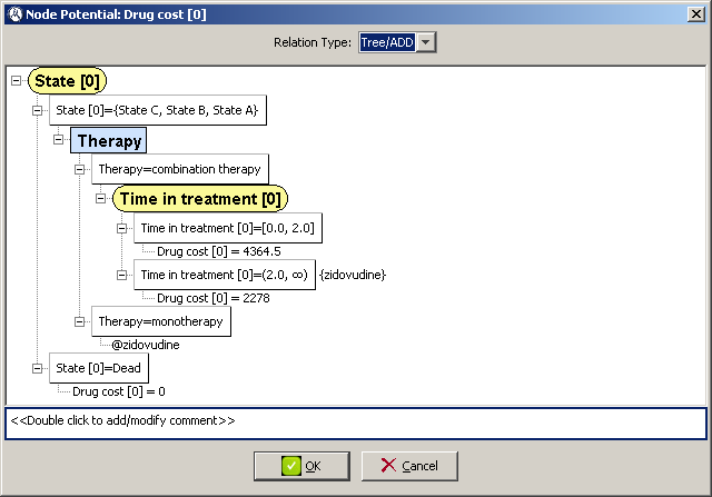
Time in treatment [1]. We might encode it as a table, but given that some of the values of that table repeat themselves, it is more appropriate to use a tree: on the contextual menu of
State [1] select
Edit probability... and choose
Tree/ADD as the
Relation type. (We will explain the meaning of ADD very soon.) A small tree will appear inside an editor----see Figure
4.2↓. The root of the tree is the first node that you declared as parent of
State [1], i.e., it depends on which link you drew first. If this root node is not
Therapy, right-click on it, click
Change variable and select
Therapy. The tree then has two branches,
monotherapy and
combined therapy. Remember that when
monotherapy is applied, the probability of the patient being in a state in cycle 1 depends on the state in cycle 0, as indicated by Table
4.1↑; it does not depend on the duration of the treatment. Consequently, right-click on the text
P(State [1]) in the
monothearpy branch, select
Add variables to potential, check the box for
State [0], and click
OK. Observe that the text has changed into
P(State [1]|
State [0]). Right-click on this text, select
Edit potential, chose
Table as the
Relation Type, introduce the transition probabilities specified in Table
4.1↑, and click
OK. This branch should look like in Figure
4.2↓.
When the treatment is
combined therapy, the probability of
State [1] depends not only on
State [0] but also
Time in treatment [1], because the patient receives zidovudine plus lamivudine for three years and then zidovudine alone, as in the case of monotherapy. Therefore, the probability of
State [1] for
combined therapy might be encoded as a three-dimensional table. However, it is better to represent it as a tree with two branches: one for the first three cycles and another one for the rest of the time, as in Figure
4.2↑. To introduce these branches, right-click on
Therapy=combined therapy and select
Add subtree and
Time in treatment [1]. This creates a subtree with a single branch that covers the whole interval
[0, ∞). Right-click on the box containing that interval, select
Split interval and
set
2 as the threshold value. Notice that the radio button
Included in the first interval is checked, which makes the threshold belong to the first sub-interval. This means that the original interval will be partitioned into
[0, 2] and
(2, ∞). Obviously, if we selected the option
Included in the second interval the partition would be
{[0, 2), [2, ∞)}. As we did in the
monotherapy branch, add the variable
State [0] to the potential
P(State [1]), right-click on the text
P(State [1]|
State [0]) in this branch, choose
Edit potential, select
Table as the
Relation Type, introduce the transition probabilities specified in Table
4.2↑, and click
OK. This branch should look like in Figure
4.2↑.
Finally, the probability of
State [1] for
combined therapy after the second year is supposed to be the same as that of
monotherapy. Therefore, it would be possible to proceed as above and copy again the values of Table
4.1↑ into a new table inside this probability tree, as in Figure
4.2↑. One disadvantage of this representation is the need to introduce the same parameters twice; if there is uncertain about a parameter, its second-order probability distribution will also have to be introduced twice. A more important disadvantage is that if a parameter changes in the light of new evidence, it will have to be updated in two places, with the risk of inconsistencies between the branches of the tree. Finally, the main drawback of this representation is that when performing sensitivity analyses OpenMarkov will sample those parameters independently, without realizing that each parameter of the model appears twice in this probability tree.
Fortunatelly, it is possible to tell OpenMarkov that two branches of the tree are the same. Properly speaking, in this case we do not have a tree, but an
algebraic decision diagram (ADD)
[21], because a node in the “tree” belongs to more than one branches. Given that trees are a particular case of ADDs, OpenMarkov and ProbModelXML have only one type of potential for both of them, called
Tree/ADD---see
[28] for a more detailed explanation.
The ADD for our example can be encoded as follows. Right-click on the node
Therapy=monotherapy in the tree, select
Add label, and write the name
tp-monotherapy, where
tp stands for “transition probabilities”. Right-click on the node
Time in treatment [1]=(2.0 ∞), select
Add reference and
tp-monotherapy, and click
OK. The result will be as shown in Figure
4.3↓
Save the network to avoid losing these changes.
The utility potential for the node
Cost [0] can also be specified as a tree/ADD. The process is very similar: in the contextual menu of this node, select
Edit utility, select
Tree/ADD as the
Relation type. Right-click on the root of the tree,
State [0], select
Change variable and choose
Therapy. In the brach
monotherapy, right-clic on
Cost [0], select
Add variables to potential and choose
State [0]. Right-click on
Cost [0](State [0]), select
Edit potential, choose
Table as
Relation type, introduce the cost associated each state, as specified in the first line of Table
4.3↑, and click
OK.
Right-clic on
Therapy=combined therapy, select
Add subtree and
Time in treatment [0]. Right-click on
Time in treatment [0]=[0.0, ∞) and select
Split interval. Set
2 as the
Threshold value and observe that the option
Included in first inverval is selected. In the branch for the interval [0.0, 2.0], right-click on
U(Cost [0]), add
State [0] as a variable, right-click on
Cost [0](State [0]), select
Edit potential, choose
Table as
Relation type, introduce the cost associated each state, as specified in the second line of Table
4.3↑, and click
OK.
Right-click on the node
Therapy=monotherapy and set the
label cost-monotherapy. Right-click on the node for the interval
(2.0,
∞) and set the
reference cost-monotherapy. The resulting potential should resemble that of Figure
4.4↓. Click
OK to save this potential.
The value of
Life years [0] given its only parent
State [0] is very simple: it is 1 for all states except for
death, which is 0. This potential can be specified as a table containing four values, but we will specify it as a tree. Right-click on
Life years [0] and choose
Edit potential from the contextual menu. Select
Tree/ADD as the
Relation type. A tree with
State [0] as the root node will appear. Right-click on the
state A branch and choose
Add states to branch in the contextual menu. In the dialog that will appear, check the boxes for
state B and
state C, and click
OK. Right-clicking on the node
Life years [0] in this branch, set the
relation type to
Table and write
1 in the only cell in the table. Next, edit the potential of the
death branch in a similar way introducing
0 in the only cell of this table. The resulting potential should look like the one in Figure
4.5↓
Save the network again.
4.2 Evaluation of the MID
The model contains all the relevant qualitative and quantitative information and is now ready for evaluation. Currently there are three ways of evaluating the model in OpenMarkov:
-
expand the network for a certain number of cycles,
-
display the evolution of a variable in time,
-
perform a cost-effectiveness analysis.
Before explaining these options in further detail, we describe the dialog used to enter the parameters for the evaluation, which is similar for the three of them.
4.2.1 Launching the evaluation
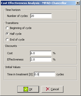
A dialog with the configurable options for the CEA will pop up like the one in Figure
4.6↓.
The configurable options for the cost-effectiveness analysis include:
-
Time horizon: The number of cycles the CEA will take into account.
-
Time of transition: Transitions can happen either at the beginning, at the end or at half cycle. The calculation of the effectiveness (usually meassured in time) will be affected by the option chosen.
-
Discounts: Usually a discount rate is applied for cost and effectiveness, which could be an very often is different.
-
Initial values: This is a list of time-dependent numeric variables in the model whose value is shifted by the cycle length in each time slice. The value for the first time slice can be set in this field.
In our example, the time horizon is 20 cycles, we will apply the half-cycle correction (i.e. transitions happen at half cycle), discount rate for cost and effectiveness will be 6% and 2% respectively and the initial value of Time in treatment will be zero (as we assume the model represents the treatment from its start point).
Hitting OK will launch the evaluation and OpenMarkov will proceed to show the results.
4.2.2 Expanding the model
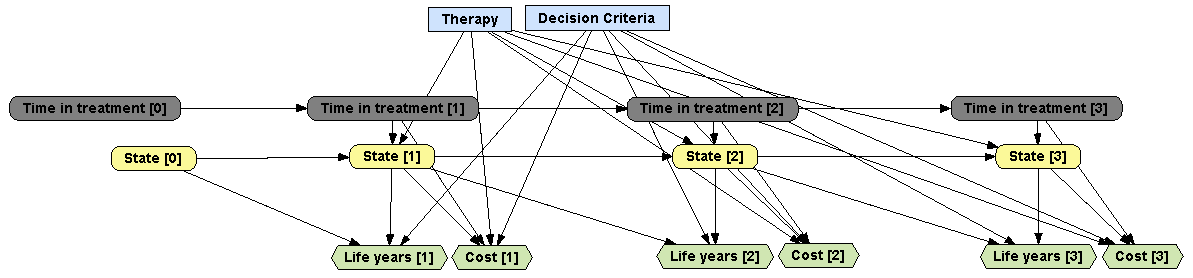
As shown in our example, when building a temporal model, i.e., a model that represents the evolution of a system over time, only the sufficient information is entered as to be able to expand the network to a variable number of cycles by creating instances of new time slices. Usually, it is enough to represent the first time slice and those variables in the second time slice that depend on the first to be able to expand a model.
In order to expand a network in
OpenMarkov, right-click on an empty spot in the network panel and choose the option
Expand Network CE in the contextual network. The options dialog described in the previous section will pop up and after entering the appropriate values (especially the number of cycles to expand) and clicking
OK, a new network panel will be opened containing the expanded MID. Figure
4.7↓ shows the MID for the Chancellor model, expanded to three cycles.
4.2.3 Temporal evolution of variables
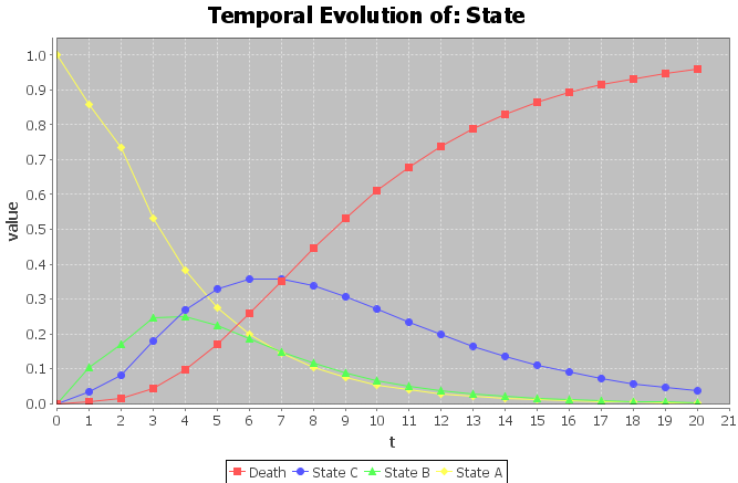
Analyzing the evolution of a variable over time can give us very useful information. In
OpenMarkov, given a strategy, the evolution of a chance or value variable can be plotted. In order to do so, first impose a policy (as described in Section
3.4↑) to each decision node in the model, then right-click on the node whose temporal evolution the user wants to analyze and choose
Temporal Evolution in the contextual menu. After introducing the evaluation parameters in the dialog described in Section
4.2.1↑, the temporal evaluation of the variable will be represented in a dialog with two tabs. The first will show a plot as the one in Figure
4.8↑, while the other will contain a table with the values of the variable in each time slice.
4.2.4 Cost-effectiveness analysis
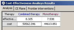
Cost-effectiveness analysis can be launched in OpenMarkov in Tools > Cost effectiveness analysis > Deterministic analysis (deterministic analysis as opposed to probabilistic analysis, described later in the tutorial).
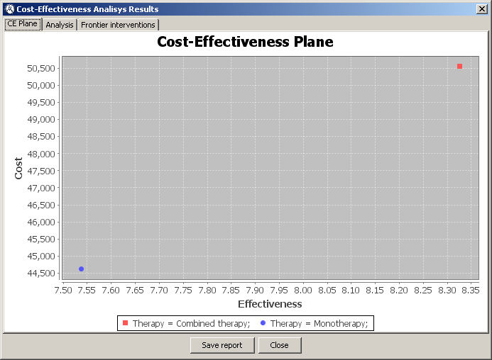
Results for deterministic cost-effectiveness analysis are separated in three tabs. The first tab shows a table containing the cost and effectiveness values for all possible strategies (also called interventions).
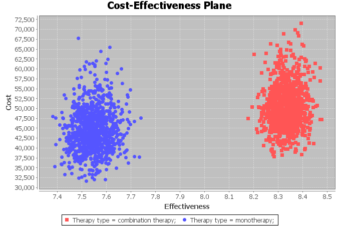
The second tab shows the cost-effectiveness plane, where cost is in the vertical axis and effectiveness is in the horizontal axis. Each intervention is represented by a point in the two-dimensional space. In our example, there is a point for monotherapy and another for combined therapy, as can be seen in Figure
4.10↓.
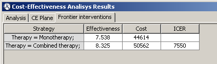
The third and last tab shows a list of frontier interventions along with the Incremental Cost-Effectiveness Ratio (also known as ICER). In our example, both interventions are frontier interventions.
4.3 Probabilistic cost-effectiveness analysis
Usually the parameters of a model (such as transition probabilities) are estimated (based on data or an expert’s knowledge) and therefore are subject to uncertainty. In order to represent this uncertainty, probability distributions are used instead of point estimates. In this section of the tutorial we will further develop our running example by setting probability distributions to some of the parameters and then we will run a probabilistic analysis based on a number of simulations.
Following with our running example of the HIV/AIDS model, let us consider that instead of having point estimates for transition probabilities in monotherapy we use Dirichlet distributions with the parameters in Table
4.4↓.
|
|
state A
|
state B
|
state C
|
|
state A
|
1251
|
-
|
-
|
|
state B
|
350
|
731
|
-
|
|
state C
|
116
|
512
|
1312
|
|
death
|
17
|
15
|
437
|
Table 4.4 withDirichlet distribution parameters for transition probabilities
Let us also consider to model direct medical and community care costs associated with each state with gamma distributions. As little information was given in the original article about the variance of costs, we will assume that the standard error is equal to the mean. Direct medical and community care costs are shown in Table
4.5↓ . Drug costs will remain fixed, £ 2278 for zidovudine and £ 2086 for lamivudine.
|
|
state A
|
state B
|
state C
|
|
Direct medical costs
|
£ 1701
|
£ 1774
|
£ 6948
|
|
Community care costs
|
£ 1055
|
£ 1278
|
£ 2059
|
Table 4.5 Direct medical and community care cost means associated with each state
4.3.1 Introducing uncertainty in the model
First, the transition probabilities need to be modified to specify that these should be drawn from a Dirichlet distribution. Right-cllick on the
State [1] node and choose
Edit probability... in the contextual menu. The dialog that will pop up should look like Figure
4.2↑. Right-click on the text
P(State [1]|State [0]) just below the
Monotherapy branch and choose
Edit potential. Right-click on any cell in the
state A column and choose
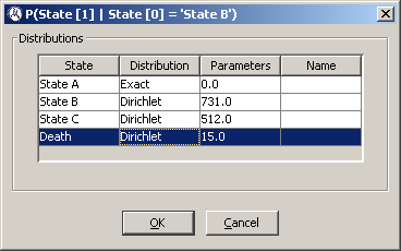
Assign uncertainty in the contextual menu and a dialog similar to that in Figure
4.12↓ will pop up. Click on the cell in the
Distribution column in the first row and choose
Dirichlet from the drop-down list. Enter the distribution’s parameter as specified in Table
4.4↑ (in this case 1251). Introduce the parameters for all transition probabilities, making sure the values specified as dashes in Table
4.4↑ are represented by Exact distributions whose parameter is zero (as in Figure
4.12↓).
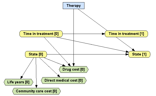
Second, the
Cost variable needs to be split into three different variables representing
Community care cost,
Direct medical cost and
Drug cost. Note that
Drug cost will have the same parents as the old
Cost node had, that is,
Therapy,
Time in treatment [0] and
State [0], but
Community care cost and
Direct medical cost will only have one parent,
State [0] as these are supposed to be the same for both therapies. The resulting MID should look as in Figure
4.12↑.
Defining the utility function for
Drug cost [0] is very similar to how we defined the utility function for the old
Cost [0] node in Section
4.1.3↑, as it contains no uncertainty. Following the same steps as in the mentioned section and with the help of Figure
4.14↓ you should be able to define
Drug cost [0]’s utility function.
Let us now use gamma distributions to define community care and direct medical costs. Right-click on
Direct medical cost [0] and choose
Edit utility... from the contextual menu. Next, select
Table from the
Relation Type drop down list. Right-click on the only cell of the
state A column and choose
Assign uncertainty from the contextual menu. Choose “
Gamma-mv” from the distribution type drop down list in the only line in the table that pops up.
OpenMarkov will then ask for the parameters of the distribution mu and sigma, i.e., the mean and the standard error, which in this case are both 1701 (as we have assumed that the standard error is equal to the mean). Do the same for
state B and
state C using the appropriate values of the first row of Table
4.5↑. The fourth state,
death, can be ignored as there is no cost attached to that state. Repeat these steps for
Community care cost [0], this time using the values of the second row of Table
4.5↑.
After doing this, the model is ready for probabilistic analysis.
4.3.2 Running the analysis
To launch the probabilistic analysis, go to
Tools > Cost effectiveness analysis > Sensitivity analysis. This will summon a dialog very similar to the one in Figure
4.6↑ but with an additional panel at the bottom to determine the number of simulations that will be run in the analysis. Clicking
OK will launch the analysis, which will usually take a few seconds; the execution time will depend on the size of the network, the number of cycles and the number of simulations.
The results of the analysis will be shown in a tabbed pane. The analysis’ summary and frontier interventions’ panels will be very similar to the ones described in Section
4.2.4↑ and are therefore no longer described here. However, the cost-effectiveness plane will have substantial differences, as the result of every simulation will be represented in the plane, and therefore each intervention will be represented as a cloud of points instead of a single point. Figure
4.15↓ shows the cost-effectiveness plane resulting from the probabilistic analysis of the Chancellor’s MID.
In addition to the panels that were present in the deterministic analysis, there are two new panels that show the results of probabilistic analysis. The first is the cost-effectiveness acceptability curve (CEAC), which represents the probability of a treatment being cost-effective (i.e. acceptable) depending on the willingness to pay, that is, the amount of money we are willing to pay for a unit in effectiveness. Figure
4.16↓ shows the CEAC resulting from the probabilistic analysis of the Chancellor’s MID. Note that there is a curve for each possible intervention, and that the probability of the less costly intervention is 1 when the willingness to pay is zero (cost is all that matters). This probability decreases and cuts the curve of the costlier (but more effective) intervention exactly at the ICER. Finally, the more effective intervention’s probability of cost-effectiveness rises to one as the willingness to pay approaches infinity.
Finally, the panel of Expected Value of Perfect Information represents the expected costs of uncertainty, as perfect information can eliminate the possibility of making the wrong decision. It is also the maximum that the health care system should be willing to pay for additional research. EVPI is calculated for the total population of patients who stand to benefit from additional information over the expected lifetime of the technology, although the EVPI for future patients is discounted at a certain rate. The graph can be customized through the parameters at the top of the chart: the max ratio (the maximum value of cost-effectiveness threshold to take into account), the population of patients, the lifetime of the technology and the discount rate.
Bibliography
[1] A. Briggs, K. Claxton, M. Sculpher: Decision Modelling for Health Economic Evaluation. Oxford University Press, 2006.
[2] A. Darwiche: Modeling and Reasoning with Bayesian Networks. Cambridge University Press, 2009.
[3] C. Lacave, M. Luque, F. J. Dı́ez: “Explanation of Bayesian networks and influence diagrams in Elvira”, IEEE Transactions on Systems, Man and Cybernetics—-Part B: Cybernetics, pp. 952-965, 2007.
[4] D. Koller, N. Friedman: Probabilistic Graphical Models: Principles and Techniques. The MIT Press, 2009.
[5] M. F. Drummond, M. J. Sculpher, G. W. Torrance, B. J. O'Brien, G. L. Stoddart: Methods for the Economic Evaluation of Health Care Programmes. Oxford University Press, 2005.
[6] E. Herskovits: Computer-based probabilistic-network construction. 1990.
[7] F. J. Dı́ez, M. J. Druzdzel: Canonical probabilistic models for knowledge engineering, 2006.
[8] F. J. Dı́ez: Introducción a los modelos gráficos probabilistas. UNED, 2007.
[9] I. A. Beinlich, H. J. Suermondt, R. M. Chávez, G. F. Cooper: “The ALARM monitoring system: A case study with two probabilistic inference techniques for belief networks”, Proceedings of the 2nd European Conference on AI and Medicine, pp. 247—256, 1989.
[10] I. Bermejo, J. Oliva, F. J. Dı́ez, M. Arias: “Interactive learning of Bayesian networks with OpenMarkov”, , pp. 27-34, .
[11] J. A. Tatman, R. D. Shachter: “Dynamic programming and influence diagrams”, IEEE Transactions on Systems, Man and Cybernetics, pp. 365—379, 1990.
[12] J. Pearl: Probabilistic Reasoning in Intelligent Systems: Networks of Plausible Inference. Morgan Kaufmann, 1988.
[13] J. V. Chancellor, A. M. Hill, C. A. Sabin, K. N. Simpson, M. Youle: “Modelling the cost effectiveness of lamivudine/zidovudine combination therapy in HIV infection.”, Pharmacoeconomics, pp. 54-66, 1997.
[14] K. B. Korb, A. E. Nicholson: Bayesian Artificial Intelligence. CRC Press, 2010.
[15] K. Ezawa: “Evidence propagation and value of evidence on influence diagrams”, Operations Research, pp. 73—83, 1998.
[16] K. P. Murphy: Machine Learning: A Probabilistic Perspective. MIT Press, 2012.
[17] S. L. Lauritzen, D. J. Spiegelhalter: “Local computations with probabilities on graphical structures and their application to expert systems”, Journal of the Royal Statistical Society, Series B, pp. 157—224, 1988.
[18] P. Spirtes, C. Glymour, R. Scheines: Causation, Prediction and Search. The MIT Press, 2000.
[19] R. A. Howard, J. E. Matheson: Influence diagrams in Readings on the Principles and Applications of Decision Analysis (R. A. Howard and J. E. Matheson, ed.). Strategic Decisions Group, 1984.
[20] R. E. Neapolitan: Learning Bayesian Networks. Prentice-Hall, 2004.
[21] R. I. Bahar, E. A. Frohm, C. M. Gaona, others: “Algebraic decision diagrams and their applications”, Proceedings of the IEEE/ACM International Conference on Computer-Aided Design (ICCAD'93), pp. 188-191, 1993.
[22] U. Kjærulff, A. L. Madsen: Bayesian Networks and Influence Diagrams: A Guide to Construction and Analysis. Springer, 2010.
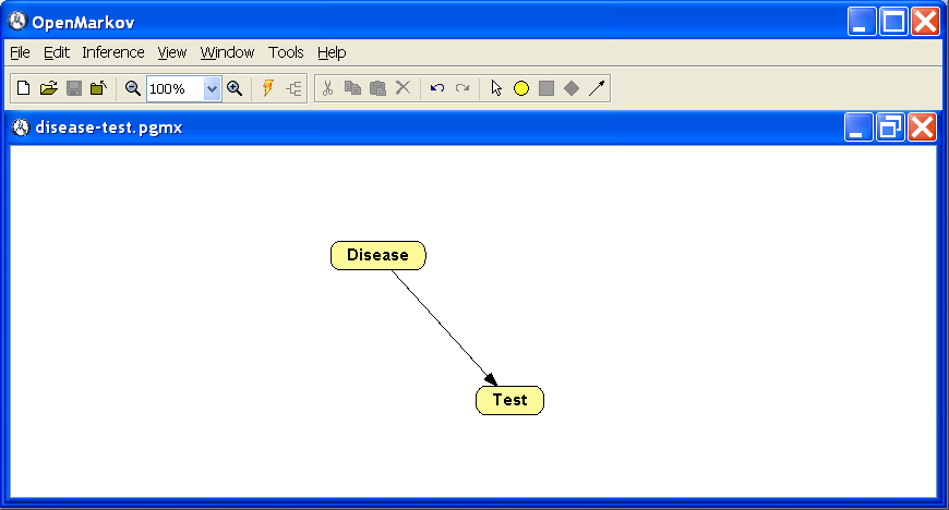
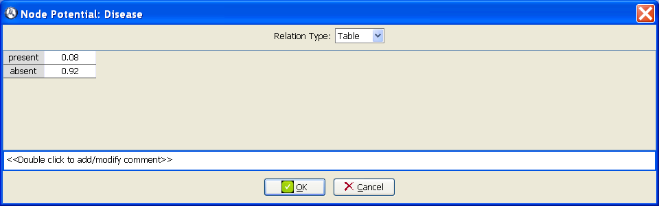
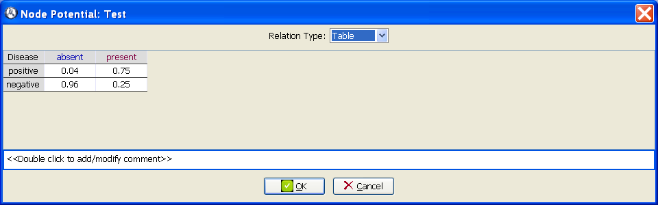
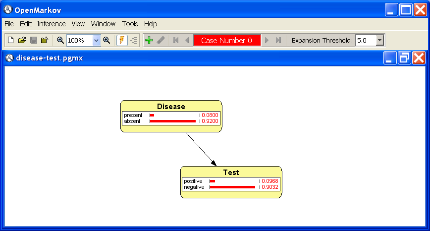
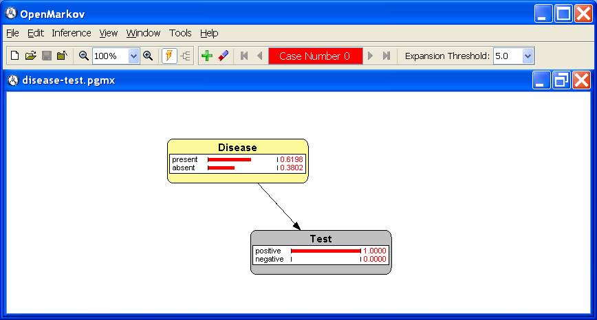
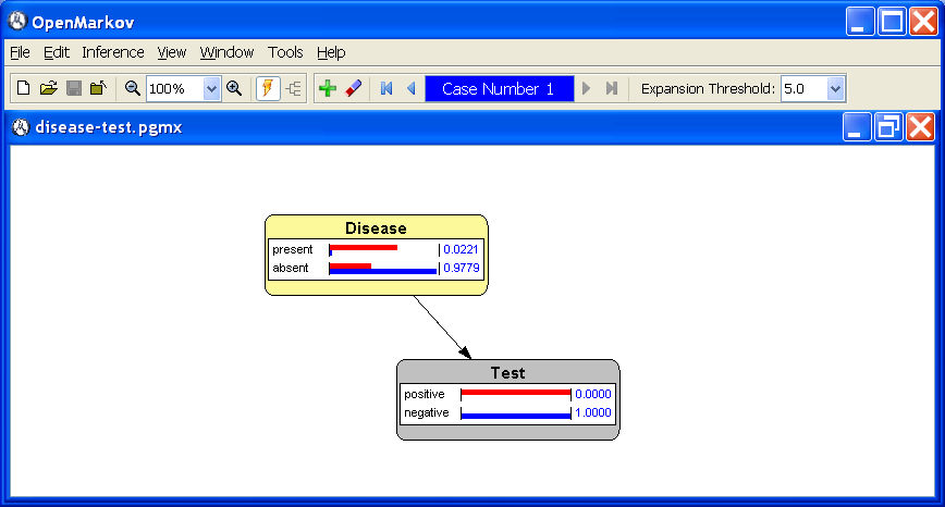
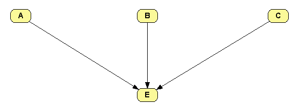
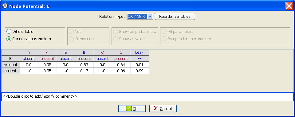
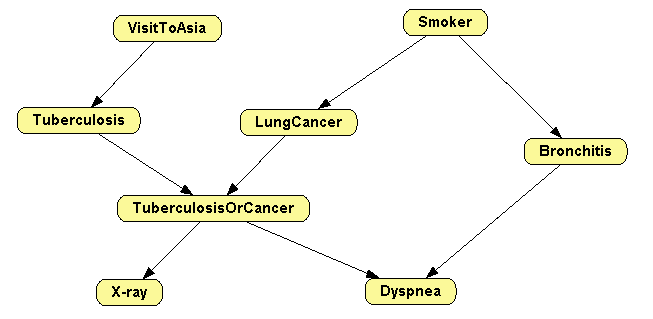
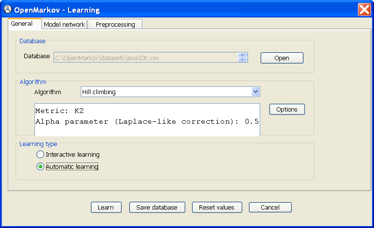
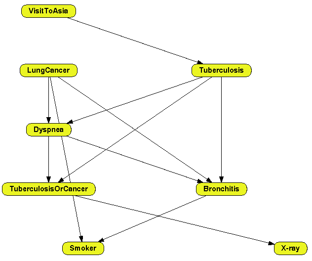
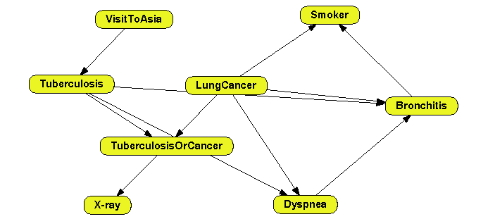
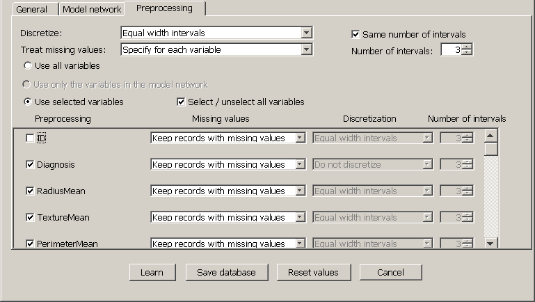
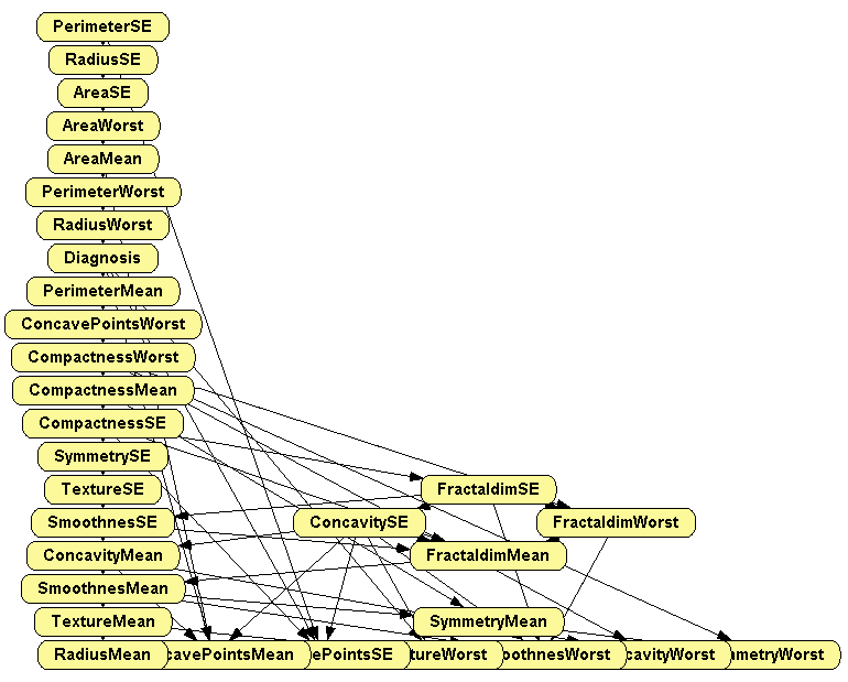
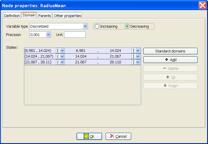
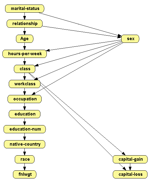
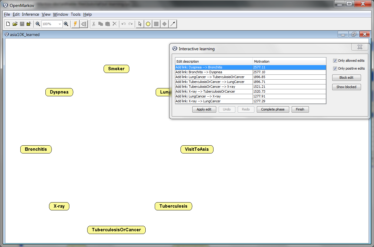
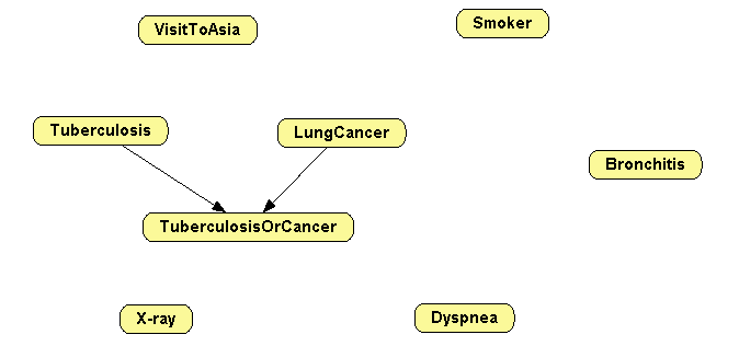
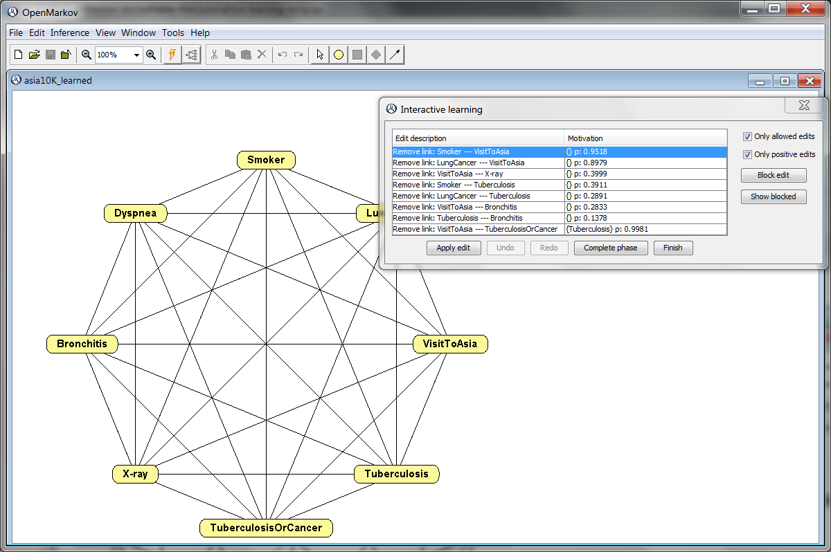
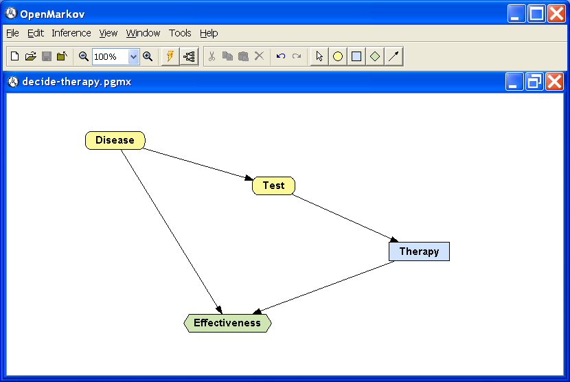
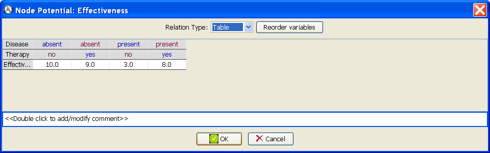
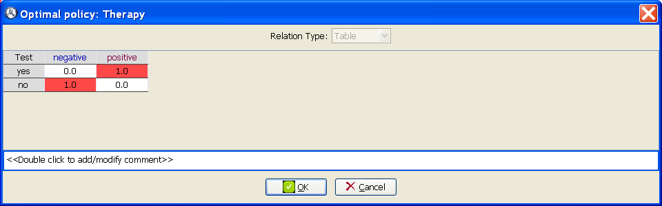
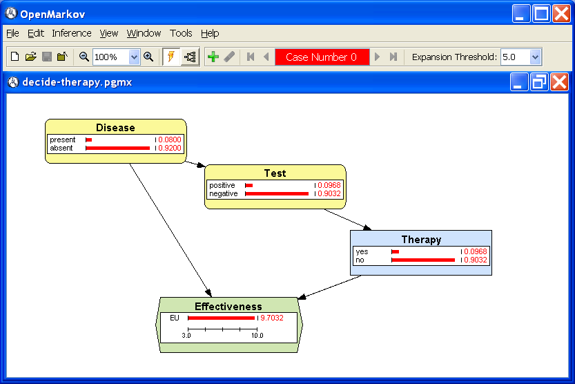
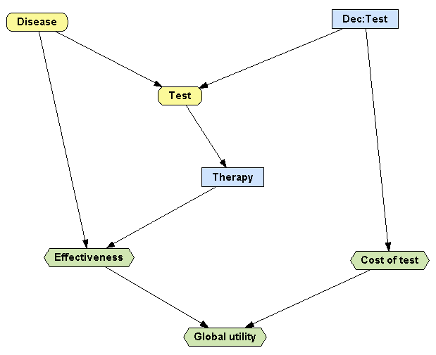
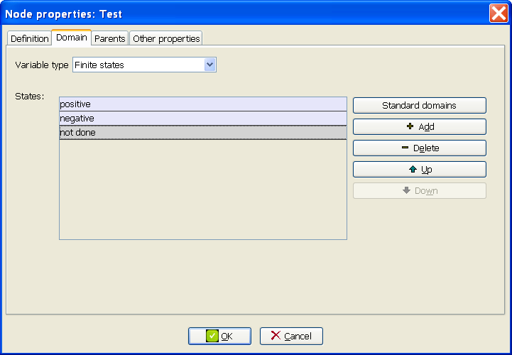
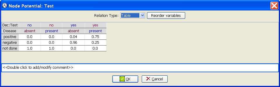
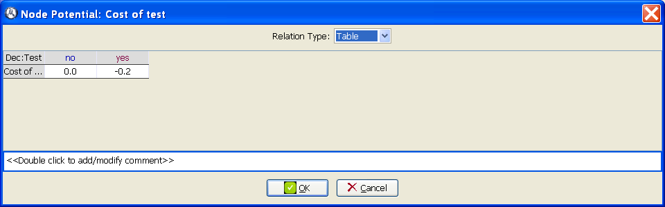
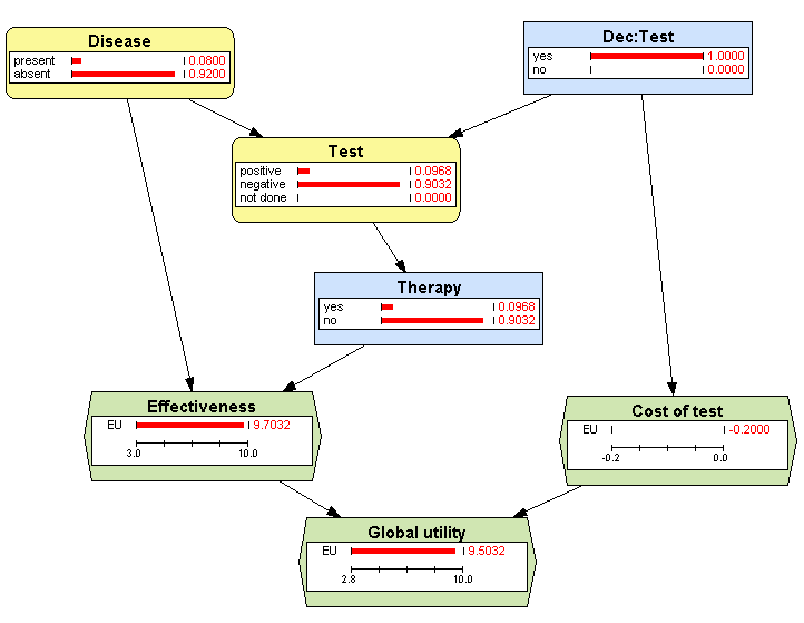
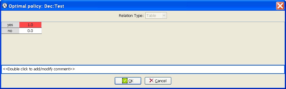
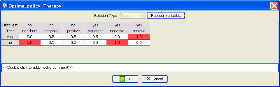
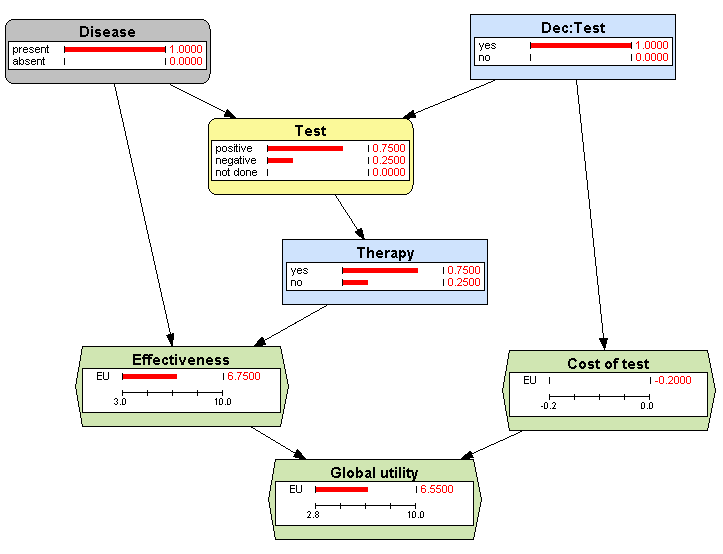
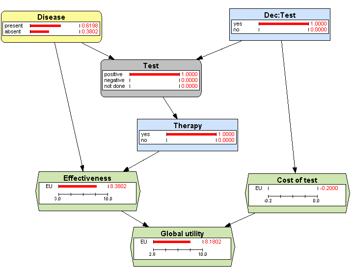
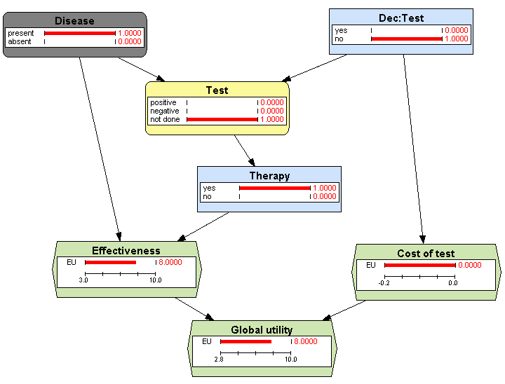
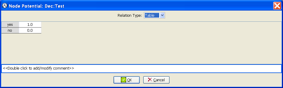
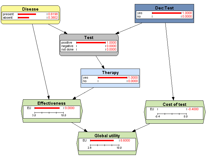
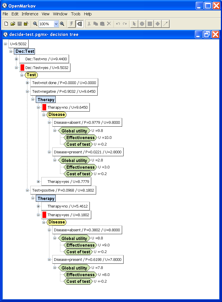
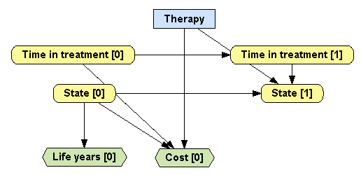
![figure float/MID-Chancellor-State[1]-tree.png](float/MID-Chancellor-State[1]-tree.png)
![figure float/MID-Chancellor-State[1].png](float/MID-Chancellor-State[1].png)
![figure float/MID-Chancellor-Cost[0].png](float/MID-Chancellor-Cost[0].png)
![figure float/MID-Chancellor-Life_years[0].png](float/MID-Chancellor-Life_years[0].png)